A monopolist is the only producer in its industry. Local utilities are a typical example. Since the monopoly is the only seller, the downward sloping industry demand curve is the monopolist's own demand curve. So to sell more the monopolist must lower its price for subsequent units. In contrast, in a perfectly competitive industry the price doesn't change as a seller increases its output, so price is equal to marginal revenue.

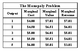
The table below illustrates this. Marginal cost is the value of the additional resources needed to produce another unit of output. The marginal benefit to consumers is the price that consumers are willing to pay for each unit. This is the consumer?s demand schedule. The economically efficient amount to produce is four, because the fourth unit is the last one for which the unit cost to the seller is less than the unit value of the buyer.

From the monopolist?s point of view though it is more profitable to produce only three units because it does not see marginal benefit the same way that buyers see it. Notice that for the seller, the extra benefit of the second unit is only $6.01. It sells the second unit for $6.51, but to sell the second unit, it had to reduce the price it charged by $.50. The price reduction from $7.01 to $6.51 reduced the revenue from the first unit by $0.50, so the net increase in its revenue was only $6.01. In a similar manner, the rest of the fourth column can be obtained.

Producing beyond the third unit is not in the interest of the monopolist. The marginal revenue of the fourth unit is only $4.01, but it costs $5.50. For market efficiency, however, the fourth unit should be produced. It brings them added benefits of $5.51 and uses resources worth only $5.50.

Graphical Representation of Monopoly

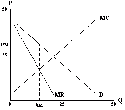
The discussion above is illustrated below. The seller chooses output q_M so that marginal cost and marginal revenue are equal. Market efficiency though occurs when output is where demand equals marginal cost (D = MC). The monopolist restricts output because of a divergence between marginal benefit as the firm perceives it and marginal benefit as buyers perceive it. Producing beyond q_M is not in the interest of the firm because the extra benefit it sees, marginal revenue, is less than the extra cost of production, shown by the marginal cost curve. Extra output is in the interest of buyers because the extra benefit they get, shown by the demand curve, is greater than the extra cost of production.

Suppose the monopolist faces the following industry inverse demand curve p = D^-1(q) = 45 - q. Then the monopolist's revenue is R(Q) = p × q = (45 - q) × q. The marginal revenue is the derivative of this function, which is MR(q) = 45 - 2 × q.

Suppose the marginal cost curve is p = MC(q) = 3 + q. Then the monopolist wants to choose the output q that equates marginal revenue and marginal cost, which is when MR(q) = 45 - 2 × q = 3 + q = MC(q). So q_M = 14.

The left hand side gives the marginal revenue from producing an extra unit of output. The right hand side gives the marginal cost of producing an extra unit of output. The monopolist produces at a quantity level where the marginal revenue equals the marginal cost.

Experiments on the monopoly model are included in MarketLink for both the double auction and the posted offer auction. If you haven't yet used MarketLink to run an experiment, go to the MarketLink page for information. If you are familiar with MarketLink, you can add these experiments to you profile from the monopoly market experiment configurations page.

Return to the IO index.