|
|
|
The Cournot model predicts that in a market with a small
number of producers, the price will fall between the price in a
competitive market and the monopoly price. To illustrate this
model, we evaluate a market with two producers.
In Cournot's original analysis, he considered the market for
mineral water in a small town, and asked what the price and
output would be if there were only two producers who compete
with each other. The total output of these two firms is the
sum of their individual outputs: Q = q1 + q2
where firm 1 produces q1 and firm 2 produces
q2.
This section describes the Cournot duopoly model as a game, and
experiment configurations are included for two versions of the game.
In a separate section, we evaluate a
duopoly market with
two sellers and several buyers.
|
|
One of the two Cournot duopoly games that we have included as an
experiment use the market demand, seller costs, and strategy sets
that were used for the duopoly experiment reported in Huck, Müller,
and Normann [2001]. The other duopoly experiment that we have
included is a simplified version of the design used by Huck, Müller,
and Normann. We start with the simplified version, because its
payoff matrix has fewer strategies.
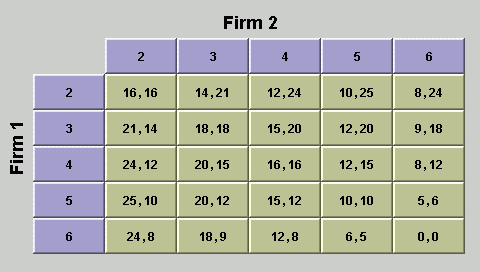
Simple duopoly game experiment
Suppose that there are two firms each with a unit cost c = 0 for each
unit produced, and the price is p = 12 - Q, where Q is the sum of the
output q1 by firm 1 and q2 by firm 2.
For the price and unit cost above, the profit function for firm 1 is
p1(q1, q2) =
(12 - q1 - q2) q1; the profit
function for firm 2 is similar:
p2(q2, q2) =
(12 - q1 - q2) q2.
Suppose also that each firm can choose one of 5 output levels,
q1 = 2, 3, 4, 5, or 6, and q2 = 2, 3, 4, 5, or 6.
The payoffs for both players are shown in the payoff table in
figure 1. The row labels represent the possible output choices by
firm 1, and the column labels represent the possible output choices
by firm 2. The first number in each cell represents the payoff to
firm 1, and the second number represents the payoff to firm 2. You
can verify that the entries in the payoff matrix are determined from
the profit functions above by calculating the values in some cells.
For example, in the cell with q1 = 4 and q2 = 3,
the price is p = 12 - q1 - q2 = 5, so the profit
of firm 1 is
p1(4, 3) =
5 × 4 = 20 and the profit function for firm 2 is
p2(4, 3) =
5 × 3 = 15.
|
|
Figure 1: Simple duopoly game payoff table
There are two things that you will want to note about the payoff table
in figure 1. First, if both firms produce 4 units (q1 = 4
and q2 = 4), then neither firm can increase its payoff
by changing its output, assuming that the other firm doesn't change
its output. This is called a
Nash
equilibrium.
Another important point is that this is not the best payoff
that can be attained by the two firms. If both firms reduce
their output to 3 (so q1 = 3 and q2 = 3)
then the profit of each firm would increase from 16 to 18. The
total profit that the two firms obtain in the Nash equilibrium,
p1 +
p2 = 32, is lower than
the maximum joint profit that they could earn,
which is p1 +
p2 = 36, because of the
competition between them.
The simple duopoly game above has only five output levels for each
choice, so the payoff table is fairly easy to understand. However,
there are two aspect of the payoff table that are undesirable.
First, not all strategies have a unique best response. Specifically,
if Firm 1 chooses 3 (or more accurately, if Firm 2 expects Firm 1 to
choose 3) then the best response by Firm 2 is to choose either 4 or
5. Similarly, if Firm 2 expects Firm 1 to choose 5, then the best response by Firm 2 is to choose either 3 or 4. Although this game
has a unique pure strategy Nash equilibrium, the formulation of the
duopoly game by Huck, Müller, and Normann has a unique best
response for each firm to each output choice by the other firm.
This proves very useful in the description of a simple dynamic of
strategy choices, so we also describe their version of the game,
and include a configuration for playing the game.
|
|
Original Huck, Müller, and Normann experiment
In the original Huck, Müller, and Normann experiment, each firm had
a unit cost of c = 6 for each unit produced, and the price is
p = 30 - Q, where Q is the sum of the output q1 by firm 1
and q2 by firm 2.
For the price and unit cost above, the profit function for firm 1 is
p1(q1, q2) =
(30 - q1 - q2) q1
- 6 q1.
The profit function for firm 2 is similar:
p2(q2, q2) =
(30 - q1 - q2) q2
- 6 q2.
In the experiment that Huck, Müller, and Normann conducted, they
only allowed output levels between 3 and 15 for each player, so
we have done the same in the experiment that we prepared. The
payoffs for both players are shown in a
payoff table.
The first number in each cell represents the payoff to firm 1, and
the second number represents the payoff to firm 2. You can verify
that the entries in the payoff matrix are determined from the profit
functions above by calculating the values in some cells. For example,
in the cell with q1 = 6 and q2 = 4, the price
is p = 20, so the profit of firm 1 is
p1(6, 4) =
20 × 6 - 6 × 6 = 84 and the profit function for firm 2 is
p2(6, 4) =
20 × 4 - 6 × 4 = 56.
|
|
As in the case of the simple duopoly game above, the Nash equilibrium
outputs (q1 = 8 and q2 = 8) lead to lower
profits for each firm that what they could obtain by colluding and
reducing outputs to q1 = 6 and q2 = 6. For
these lower output levels, the profit of each firm would increase from
64 to 72. The
total profit that the two firms obtain in the Nash equilibrium,
p1 +
p2 = 128, is lower than
the maximum joint profit that they could earn,
which is p1 +
p2 = 144.
|
|
If you are familiar with how to run experiments on EconPort, you can
click on one of the buttons below to add the experiment to your
EconPort profile. If you haven't previously run an EconPort experiment,
read about
EconPort Configuration and Experiment Setup before you install a
configuration.
To include the simple duopoly game in your EconPort experiment
configuration profile, click on the button below.
|
|
To include the Huck, Müller, and Normann duopoly game in your EconPort
experiment configuration profile, click on the button below.
|
|
References
Cournot, Antoine Augustin (1838). "Recherches sur les principes
mathématiques de la théorie des richesses," (translated by N.T.
Bacon as Researches into the Mathematical Principles of the Theory
of Wealth, 1897).
Huck, Steffan, Wieland Müller, and Hans-Theo Normann (2001).
"Stackelberg beats Cournot: On collusion and effciency in
experimental markets," Economic Journal 111, pp. 749-766.
|
|
Return to the IO index.
|
| |
|
|
|

 Printer Friendly


;)